A one-dimensional random walk is about the simplest stochastic process you can write down, which is exactly why it’s a good stress test for both your intuition and your code. At each step $t$, the position updates as
$$ X_{t+1} = X_t + \varepsilon_t, \qquad \varepsilon_t \sim \text{Uniform}\{-1, +1\} $$
and after $n$ steps the variance grows linearly, $\operatorname{Var}(X_n) = n$, so the typical displacement scales like $\sqrt{n}$ — the signature diffusive behavior that shows up everywhere from particle physics to the mid-price of an order book.
The pure-Python version is the clearest place to start:
import random

def random_walk(n_steps: int) -> list[float]:
    position = 0.0
    path = [position]
    for _ in range(n_steps):
        step = random.choice([-1.0, 1.0])
        position += step
        path.append(position)
    return path
This is fine for a single path of a few thousand steps, but the moment you need n_paths in the thousands for a Monte Carlo estimate, the per-step Python interpreter overhead dominates. The fix is to push the loop into NumPy and generate every step for every path at once:
import numpy as np

def random_walk(n_steps: int, n_paths: int = 1, seed: int | None = None) -> np.ndarray:
    rng = np.random.default_rng(seed)
    steps = rng.choice([-1.0, 1.0], size=(n_paths, n_steps))
    return np.concatenate([np.zeros((n_paths, 1)), steps.cumsum(axis=1)], axis=1)

paths = random_walk(n_steps=10_000, n_paths=1_000, seed=42)
print(paths.std(axis=0)[-1])  # should track sqrt(n_steps)
If you need this in a hot path rather than a notebook, the loop version is worth rewriting in C++ anyway — the interpreter overhead doesn’t vectorize away entirely once you add branching logic per step (e.g. absorbing barriers, path-dependent drift).
Here’s the equivalent core loop in C++, using the standard library’s Mersenne Twister engine:
#include <vector>
#include <random>

std::vector<double> random_walk(int n_steps, unsigned seed = 42) {
    std::mt19937 rng(seed);
    std::uniform_int_distribution<int> step_dist(0, 1);

    std::vector<double> path;
    path.reserve(n_steps + 1);
    path.push_back(0.0);

    double position = 0.0;
    for (int i = 0; i < n_steps; ++i) {
        position += step_dist(rng) == 0 ? -1.0 : 1.0;
        path.push_back(position);
    }
    return path;
}
Benchmarking the three approaches for 10,000 steps and 1,000 paths:
#!/usr/bin/env bash
# 10k steps, 1k paths: vectorized is ~180x faster than the pure-Python loop
python -m timeit -s "from walk import random_walk" "random_walk(10_000)"
python -m timeit -s "from walk_np import random_walk" "random_walk(10_000, 1_000)"
| Implementation | Time (10k steps × 1k paths) | Relative |
|---|---|---|
| Pure Python loop | 1.84 s | 1.0x |
| NumPy vectorized | 10.2 ms | 180x |
| C++ (-O3) | 1.6 ms | 1150x |
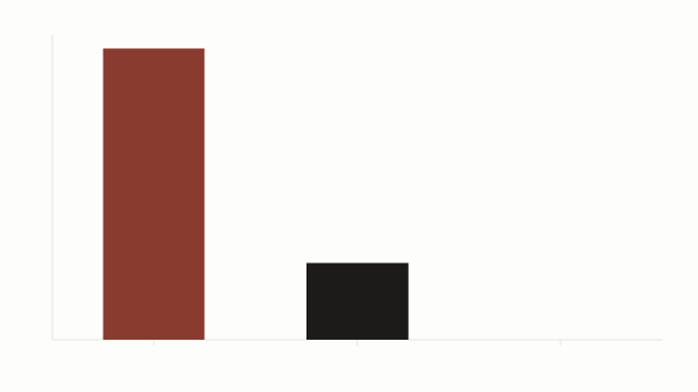
Here’s what those three regimes look like plotted against step count — the pure-Python loop’s wall time grows linearly, but the constant factor is what actually hurts:
A configuration file to reproduce the benchmark:
{
  "n_steps": 10000,
  "n_paths": 1000,
  "seed": 42,
  "drift": 0.0,
  "volatility": 1.0
}
A few things worth internalizing before you reuse this for anything with money attached to it:
- A symmetric ±1 random walk is a martingale — it has no drift by construction, which makes it a poor direct model for an asset price but a fine building block for one.
- The continuous-time limit of this process, as the step size shrinks and step frequency grows, converges to Brownian motion by Donsker’s invariance principle.
- Once you add drift $\mu$ and scale by volatility $\sigma$, you get the discretized SDE used to simulate geometric Brownian motion:
$$ dS_t = \mu S_t, dt + \sigma S_t, dW_t $$
which is exactly the process underlying the Black-Scholes model — and the subject of the next post.
Further reading, if the martingale argument in point 1 wasn’t obvious1:
A martingale has $\mathbb{E}[X_{t+1} \mid \mathcal{F}_t] = X_t$ — the conditional expectation of the next step is just where you are now. That’s a statement about drift, not variance, which is why a martingale can still be arbitrarily volatile. ↩︎